From Linear Attention to Test-Time Training

This blog post is based on the CVPR 2026 paper ViT $^3$ : Unlocking Test-Time Training in Vision.

In this post, we explore the connection between attention and sequence modeling, and how it leads to a new paradigm called test-time training (TTT). First, let’s start with a brief review of standard softmax attention and linear attention.

Softmax Attention

Let $Q, K \in \mathbb{R}^{N \times d_k}$ be the query and key matrices, and let $V \in \mathbb{R}^{N \times d_v}$ be the value matrix. Standard scaled dot-product attention is

O = \operatorname{softmax}\left(\frac{QK^T}{\sqrt{d_k}}\right)V,

where the softmax is applied row-wise. Computing all pairwise query-key scores is $O(N^2 d_k)$ , and mixing the values is $O(N^2 d_v)$ . We usually summarize this as $O(N^2 d)$ : the quadratic dependence on $N$ makes long contexts expensive.

Linear Attention

Linear attention replaces the softmax similarity with a factorized kernel. It uses a feature map $\phi: \mathbb{R}^{d_k} \to \mathbb{R}^{r}$ , applied row-wise to $Q$ and $K$ , to define

\kappa(q_i, k_j) = \phi(q_i)^T \phi(k_j), \quad \forall i,j.

In some variants, $\kappa$ approximates the exponential softmax kernel; in others, it is a different kernel chosen for efficiency.

Substituting this into the attention formula gives:

\begin{aligned} o_i &= \frac{\sum_{j=1}^{N} \phi(q_i)^T \phi(k_j) v_j}{\sum_{j=1}^{N} \phi(q_i)^T \phi(k_j)}, \\ &= \frac{\phi(q_i)^T \left(\sum_{j=1}^{N} \phi(k_j) v_j^T\right)}{\phi(q_i)^T \left(\sum_{j=1}^{N} \phi(k_j)\right)}, \\ &= \frac{\phi(q_i)^T S}{\phi(q_i)^T z}, \end{aligned}

where

S = \sum_{j=1}^{N} \phi(k_j) v_j^T, \qquad z = \sum_{j=1}^{N} \phi(k_j).

Here, $S$ is a fixed-size summary of the key-value pairs, while $z$ acts as a normalization term.

Here, $S \in \mathbb{R}^{r \times d_v}$ , $z \in \mathbb{R}^{r}$ , and $o_i \in \mathbb{R}^{d_v}$ . Once $S$ and $z$ have been computed, evaluating one output costs $O(r d_v)$ . Computing all outputs therefore costs $O(N r d_v)$ . In the common case $r = d_v = d$ , this becomes $O(Nd^2)$ : linear in the sequence length $N$ .

This kernel-based formulation is described in Transformers are RNNs: Fast Autoregressive Transformers with Linear Attention.

Causal Linear Attention

In autoregressive generation, only a prefix of the sequence is visible, and the sequence grows over time. Linear attention can maintain the corresponding summary incrementally:

\begin{aligned} S_t &= \sum_{j=1}^{t}\phi(k_j)v_j^T, \\ z_t &= \sum_{j=1}^{t}\phi(k_j). \end{aligned}

Constructing the summary for a prefix of length $t$ costs $O(t d^2)$ when $r = d_v = d$ . Each new token then updates the state as follows:

\begin{aligned} S_{t+1} &= S_t + \phi(k_{t+1})v_{t+1}^T, \\ z_{t+1} &= z_t + \phi(k_{t+1}). \end{aligned}

Each update costs $O(d^2)$ , so processing a sequence of length $N$ remains $O(Nd^2)$ overall.

A Different View of Attention

We can reformulate the two types of attention in the following way. When $K$ and $V$ are fixed, softmax attention computes

O = \sigma(QK^T)V,

where $Q$ can be viewed as an input to the linear layer $K^T$ , followed by a softmax activation, and then a linear layer $V$ without activation. This is a two-layer MLP with a nonlinearity in between.

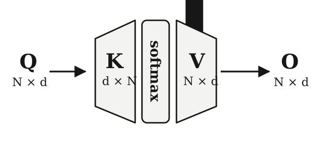
Softmax attention as a two-layer MLP: Q is multiplied by K transpose, normalized with softmax, and multiplied by V to produce O.

For linear attention, we can consider the simplest unnormalized form, and deliberately omitting the feature map. By associativity, we have

O = (QK^T)V = Q(K^TV).

Similarly, we can consider $Q$ as an input to a linear layer $K^T V$ (whose weights can be precomputed), without any intervening activation. This is a single-layer MLP.

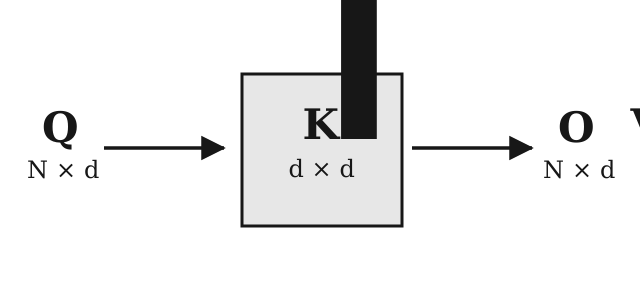
Linear attention as a single-layer MLP: Q is multiplied by the precomputed K transpose V summary to produce O.

The pattern is clear: build a model with $K$ and $V$ as parameters, then apply the model to $Q$ to get the output. This is an important reformulation of the attention mechanism.

The MLP in the middle can be viewed as a sequence-modeling function. Under this perspective, the key difference between softmax and linear attention is that softmax attention keeps the individual keys and values available to each query, whereas linear attention first reduces them to a fixed-size summary. This compression makes linear attention more efficient, but can limit the information available to each query.

Sequence modelling can therefore be viewed as a compression problem: build a compact representation of the observed sequence, then use it to predict future tokens. The central trade-off is between the fidelity of that representation and the cost of constructing and evaluating it. Naturally, one might ask: can we learn a compression function more expressive than the hand-designed linear attention while still keeping the cost linear?

One possible answer is to use a neural network. Self-supervised learning can encode a large training set in model weights while capturing useful structures and relationships in the data. This idea leads to the concept of Test-Time Training (TTT).

The connection between attention and an inner learner was introduced in Learning to (Learn at Test Time) and was further developed in Learning to (Learn at Test Time): RNNs with Expressive Hidden States.

The Test-Time Training Paradigm

TTT treats the key-value pairs as a small dataset. At inference time, an inner model is optimized to map $K$ to $V$ using a loss $\mathcal{L}(\hat{V}, V)$ , thereby compressing the current sequence into its parameters. The queries $Q$ are then fed to this adapted model to produce $O$ . Because this optimization happens during inference, it is called test-time training.

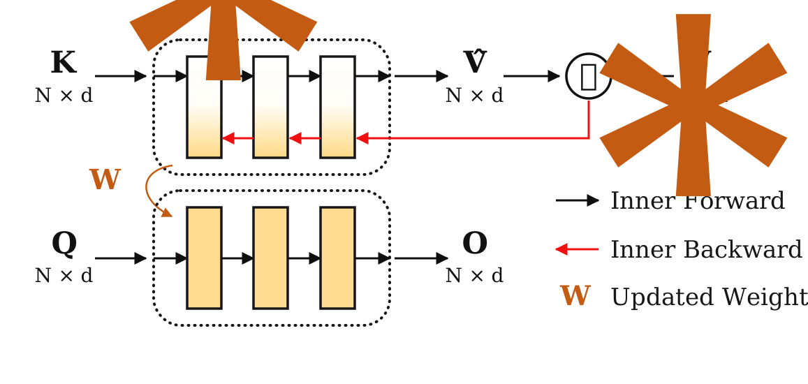
Formally, let $f(\cdot; W)$ be the inner model with temporary parameters $W$ . A full-sequence inner-model update can be written as

W' = W - \eta \nabla_W \sum_{i=1}^{N} \mathcal{L}\left(f(k_i; W), v_i\right), \qquad O = f(Q; W').

The update aims to compress the current sequence into $W'$ . In a causal setting, the same idea updates the state from each growing prefix:

W_t = W_{t-1} - \eta \nabla_W \mathcal{L}\left(f(k_t; W_{t-1}), v_t\right), \qquad o_t = f(q_t; W_t).

The Outer Loop

During ordinary training, the outer loop optimizes the task loss, but in order to do so, it must also “optimize” the inner loop. It learns the projections that produce $Q$ , $K$ , and $V$ , sometimes along with the inner-model initialization $W_0$ — these all affect the inner-loop optimization.

At deployment, outer-loop parameters are frozen, while the inner model is adapted to each new sequence at test time. The outer loop is therefore, in some sense, a meta-learning objective: it learns parameters that make the inner-loop adaptation more effective.

In principle, the inner model can be any differentiable neural-network architecture, which creates a large design space. ViT $^3$ : Unlocking Test-Time Training in Vision studies this design space for vision.

Practical Limitation

TTT avoids materializing all $N^2$ query-key interactions, but linear scaling in $N$ does not make it free. A linear inner model still typically costs $O(Nd^2)$ and, because it is adapted at runtime, also requires a backward pass, which significantly increases the computational burden and puts pressure on memory throughput. The inner model must therefore be small enough to be practical, and the outer loop must learn an initialization that makes the inner model effective with only a few gradient steps.