Paper walkthrough

Self-Distillation Enables Continual Learning
Self-Distillation Fine-Tuning (SDFT)

SDFT uses a demonstration-conditioned version of itself as teacher, turning expert demonstrations into on-policy signals. It learns new tasks while forgetting much less than SFT.

Idan Shenfeld, Mehul Damani, Jonas Hübotter, Pulkit Agrawal · MIT, Improbable AI Lab, ETH Zurich
arXiv 2601.19897v2 (2026-08-07) · Code: github.com/Continual-Intelligence/Self-Distillation

65.4 vs 56.0
Prior-task average after Tool Use training: SDFT vs SFT (base 65.5)
70.6 vs 63.2
Tool Use accuracy: SDFT vs SFT (base 42.9)
98 vs 80
OOD accuracy on newly injected 2025 facts: SDFT vs SFT

On-policy learning forgets less, but usually needs rewards

With demonstrations alone, the default is SFT, an off-policy method.

The core tension

  • Continual learning: acquire skills and knowledge without degrading existing capabilities. Deployed models currently keep their parameters fixed.
  • On-policy training (learning from the model's own samples) reduces forgetting relative to off-policy training (RL's Razor, Shenfeld et al. 2025; Chen et al. 2025) and improves generalization (Chu et al. 2025).
  • Most successful on-policy methods use reinforcement learning, requiring explicit rewards that many real-world settings lack.
  • Learning from demonstrations mainly uses SFT: training on a fixed expert distribution leads to compounding errors at inference (Ross et al. 2011) and catastrophic forgetting.

Question: How can we learn on-policy from demonstrations alone?

Existing approaches and their limits

  • Inverse RL(IRL):Infer a reward, then run on-policy RL. Strong structural priors (maximum entropy, adversarial discriminators, preference pairs) are needed; otherwise the problem is ill-posed or too costly.
  • Context distillation (Bai et al. 2022; Snell et al. 2022): a model with extra context teaches itself without that context. Usually offline, trained on teacher samples, with fixed context (e.g., guidelines or few-shot examples).

What SDFT changes

  • Distillation is on-policy: the student trains on its own trajectories, letting the teacher correct errors where they arise.
  • Teacher context is a demonstration specific to each query, rather than a global prefix, expressing fine-grained task intent.
  • The pretrained model's in-context learning (ICL) replaces an explicit reward model.
  • Concurrent independent work proposed similar self-distillation: Zhao et al. 2026; Hübotter et al. 2026 ("RL via self-distillation").

Two modes: the teacher stays closer to the base than SFT

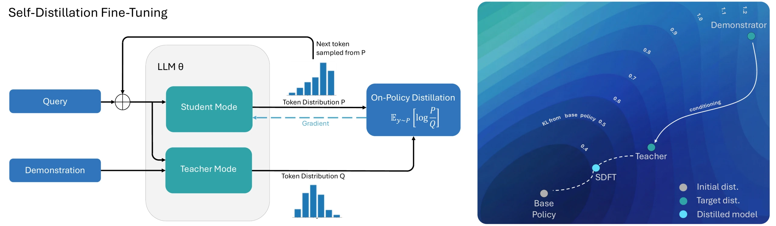
Left: SDFT pipeline. Right: demonstration conditioning stays closer to the base distribution at the same new-task accuracy.

Figure 2: SDFT pipeline and policy distributions
Figure 2 in the paper. Left: the query enters student mode to sample tokens; the same LLM in teacher mode also sees a demonstration. KL between token distributions $P$ and $Q$ provides the gradient. Right: SDFT stays closer to the base policy than SFT while reaching the target region near the demonstrator.

Student mode

Sees only query $x$ and samples $y\sim\pi_\theta(\cdot\mid x)$. All training trajectories come from this mode: on-policy.

Teacher mode

The same model (EMA weights) also sees demonstration $c$, producing $\pi(\cdot\mid y_{\lt t},x,c)$ at each student-generated position.

Key measurement (§3.2)

KL to base: teacher 0.68 nats, SFT 1.26 nats, at the same new-task accuracy.

One model takes two roles

The teacher also sees the demonstration; the student sees only the query and generates training trajectories.

Roles

Student$P=\pi_\theta(\cdot\mid x)$
Query only
Sample response $y$
On $y$,
match teacher
←
Teacher$Q=\pi(\cdot\mid x,c)$
Same model + demonstration $c$
Score student tokens

Teacher prompt (verbatim)

<Question>
This is an example for a response to the question:
<Demonstration>
Now answer with a response of your own, including the thinking process:

The authors find this prompt prevents copying $c$ verbatim: the teacher generates its own response, reflecting its understanding of the demonstration's intent.

Notation

  • $\theta$: student parameters, the only ones that receive gradients. Their value at step $k$ is $\theta_k$, abbreviated $\pi_k\equiv\pi_{\theta_k}$ (used on the next two slides).
  • The teacher $\pi(\cdot\mid x,c)$ is a constant in the loss. In the derivation it shares the student's parameters $\theta_k$; in the implementation it uses EMA parameters $\phi$, i.e. $\pi_\phi(\cdot\mid x,c)$ (algorithm on the next slide).

Objective

Sample $y$ from the student and minimize student-to-teacher KL:

$$\mathcal{L}(\theta)=D_{\mathrm{KL}}\big(\pi_\theta(\cdot\mid x)\,\|\,\pi(\cdot\mid x,c)\big)=\mathbb{E}_{y\sim\pi_\theta(\cdot\mid x)}\left[\log\frac{\pi_\theta(y\mid x)}{\pi(y\mid x,c)}\right]$$(1)

Step 1: differentiate (1). $\theta$ appears in both the sampling distribution and the log ratio. The score-function identity $\nabla\pi_\theta=\pi_\theta\nabla\log\pi_\theta$ handles the former; the latter contributes $\mathbb{E}_{y\sim\pi_\theta}[\nabla_\theta\log\pi_\theta(y\mid x)]=0$:

$$\nabla_\theta\mathcal{L}=\mathbb{E}_{y\sim\pi_\theta}\left[\log\frac{\pi_\theta(y\mid x)}{\pi(y\mid x,c)}\,\nabla_\theta\log\pi_\theta(y\mid x)\right]$$(2a)

Step 2: approximate per token. $\log\pi(y\mid x)=\sum_t\log\pi(y_t\mid y_{\lt t},x)$. At each position the paper keeps only that position's KL, summed exactly over the vocabulary $\mathcal{V}$ (the analytic per-token estimator):

$$g=\mathbb{E}_{y\sim\pi_\theta}\sum_t\sum_{y_t\in\mathcal{V}}\pi_\theta(y_t\mid y_{\lt t},x)\,\log\frac{\pi_\theta(y_t\mid y_{\lt t},x)}{\pi(y_t\mid y_{\lt t},x,c)}\,\nabla_\theta\log\pi_\theta(y_t\mid y_{\lt t},x)$$(2)

(2) is not (2a): it drops how $y_t$ changes the ratios of later tokens, which amounts to minimizing $\sum_t D_{\mathrm{KL}}$ on fixed student prefixes. This is the sequence-level bias noted in Appendix A.1.

  • Supervision is dense: every token, over the full vocabulary, from one rollout per query; GRPO-style methods give one advantage per trajectory and need a group of samples.
  • The theory uses reverse KL, but forward KL works best in practice; the repository README (2026-04-07) says all paper results use per-token forward KL.

Algorithm and key design choices

Each choice is either ablated in the appendix or used by default in the main experiments.

Algorithm 1 (SDFT)

Initialize teacher weights $\phi\leftarrow\theta$
For each training step:
Sample demonstration minibatch $\{(x_i,c_i)\}$
For each pair in parallel:
$y_i\sim\pi_\theta(\cdot\mid \mathrm{Ctx}_S(x_i))$ — on-policy rollout
$\ell^S_{i,t}\leftarrow\log\pi_\theta(y_{i,t}\mid y_{i,\lt t},\mathrm{Ctx}_S(x_i))$
$\ell^T_{i,t}\leftarrow\log\pi_\phi(y_{i,t}\mid y_{i,\lt t},\mathrm{Ctx}_T(x_i,c_i))$
$g\leftarrow$ analytic per-token KL gradient, averaged over $i$
Optionally use importance sampling for inference/training engine differences
$\theta\leftarrow\theta-\eta\,g$
$\phi\leftarrow\alpha\,\theta+(1-\alpha)\,\phi$ — EMA teacher

Teacher weights (Appendix A.3)

  • Frozen base model: stable but weaker; it cannot track the student's improvements.
  • Current student directly: unstable; small fluctuations are amplified by the on-policy loop, causing divergence.
  • EMA of student weights ($\alpha\in\{0.01,0.02,0.05\}$): tracks progress and smooths updates. Default choice.

KL gradient estimator (Appendix A.1)

  • Sampled token-level estimator:Higher variance and weaker KL control.
  • Analytic per-token estimator (sum over vocabulary at each step): biased at sequence level, but most stable and effective. Default choice.
  • Rao-Blackwellized estimator (unbiased): extra cost without measurable gains.
  • Multiple rollouts per query: negligible gains with much more compute.

Suppressing artifacts (§5)

Students may learn teacher phrases such as "Based on the text…". Masking loss on the first few tokens removes these without harming accuracy.

An inverse RL view: demonstrations define an implicit reward

Under an assumption, self-distillation is equivalent to on-policy RL with rewards supplied by the model's own ICL.

Derivation (§3.1)

  1. One trust-region RL update ($\pi_k=\pi_{\theta_k}$ is the current student; $\pi$ ranges over all policies):
    $$\pi_{k+1}=\arg\max_{\pi}\ \mathbb{E}_{y\sim\pi}\big[r(y,x)\big]-\beta\,D_{\mathrm{KL}}\big(\pi(\cdot\mid x)\,\|\,\pi_k(\cdot\mid x)\big)$$(3)
  2. The closed-form optimum is a tilted distribution $\pi^*_{k+1}(y\mid x)\propto\pi_k(y\mid x)\,e^{r(y,x)/\beta}$, hence
    $$r(y,x)=\beta\big[\log\pi^*_{k+1}(y\mid x)-\log\pi_k(y\mid x)\big]+C$$
  3. In-context assumption: The same model (parameters $\theta_k$), conditioned on the demonstration, approximates the unknown optimal policy
    $$\pi^*_{k+1}(y\mid x)\approx\pi(y\mid x,c)$$(4)
  4. Implicit reward (dropping $\beta$ and $C$) and its per-token form, which sums to the sequence reward:
    $$r(y,x,c)=\log\frac{\pi(y\mid x,c)}{\pi_k(y\mid x)},\qquad r_t=\log\frac{\pi(y_t\mid y_{\lt t},x,c)}{\pi_k(y_t\mid y_{\lt t},x)}$$(5)
  5. Policy gradient (evaluated at $\theta=\theta_k$, reward held fixed)
    $$\nabla_\theta J\big|_{\theta_k}=\mathbb{E}_{y\sim\pi_k}\left[\log\frac{\pi(y\mid x,c)}{\pi_k(y\mid x)}\,\nabla_\theta\log\pi_\theta(y\mid x)\big|_{\theta_k}\right]$$(6)
    This is exactly the negative of Equation (2a) at $\theta=\theta_k$: maximizing this reward minimizes reverse KL. The implemented Equation (2) is a per-token approximation of (2a).

Interpretation

  • The student is rewarded for approaching its more informed, demonstration-conditioned self.
  • No reward model or explicit reward prior is required: the prior is the pretrained model's ICL ability.
  • The trust-region term explains anchoring: the target is the high-reward policy closest to the current model. This starts the forgetting argument on the next two slides.

Caution

This equivalence concerns reverse KL. Experiments use forward KL, so the IRL argument motivates the method rather than exactly describing the implemented loss.

Why less forgetting? (I) The ideal target changes as little as needed

The paper gives no forgetting bound. Its argument has three links; only the first is rigorous mathematics.

① Trust-region optimum = minimum KL change MathThe tilted distribution is closest to $\pi_k$ among policies reaching a given reward.
+
② Demonstration-conditioned teacher ≈ optimum Assumption$\pi(\cdot\mid x,c)\approx\pi^*_{k+1}$, and similarly close to $\pi_k$.
+
③ Small new-task KL ⇒ less forgetting EmpiricalFrom prior work including RL's Razor; not derived here.

① The optimum's minimum-change property

"High reward, but not far from $\pi_k$" can be written two ways. Equation (3) puts a price $\beta$ on change. Alternatively, set a passing mark $v$ for reward and pick the passing policy that changes least:

$$\min_{\pi}\ D_{\mathrm{KL}}\big(\pi\,\|\,\pi_k\big)\quad\text{s.t.}\quad\mathbb{E}_{y\sim\pi}\big[r(y,x)\big]\ge v$$

With $v=\mathbb{E}_{\pi^*_{k+1}}[r]$, the reward of Equation (3)'s optimum $\pi^*_{k+1}=\pi_k\,e^{r/\beta}/Z$ (normalizer $Z=\sum_y\pi_k(y\mid x)\,e^{r(y,x)/\beta}$), both give the same answer. Taking logs gives $\log\frac{\pi^*_{k+1}}{\pi_k}=\frac{r}{\beta}-\log Z$. For any $\pi$:

$$\begin{aligned}D_{\mathrm{KL}}(\pi\,\|\,\pi_k)&=\mathbb{E}_{\pi}\Big[\log\frac{\pi}{\pi_k}\Big]&&\text{definition of KL}\\&=\mathbb{E}_{\pi}\Big[\log\frac{\pi}{\pi^*_{k+1}}\Big]+\mathbb{E}_{\pi}\Big[\log\frac{\pi^*_{k+1}}{\pi_k}\Big]&&\text{multiply and divide by }\pi^*_{k+1}\\&=D_{\mathrm{KL}}(\pi\,\|\,\pi^*_{k+1})+\mathbb{E}_{\pi}\Big[\frac{r}{\beta}-\log Z\Big]&&\text{a KL; substitute the log ratio}\\&=\underbrace{D_{\mathrm{KL}}(\pi\,\|\,\pi^*_{k+1})}_{\ge 0,\ =0\iff\pi=\pi^*_{k+1}}+\frac{\mathbb{E}_{\pi}[r]}{\beta}-\log Z&&Z\text{ does not depend on }y\end{aligned}$$

At $\pi=\pi^*_{k+1}$ the first term is 0, so $D_{\mathrm{KL}}(\pi^*_{k+1}\,\|\,\pi_k)=v/\beta-\log Z$. A passing $\pi$ has $\mathbb{E}_\pi[r]\ge v$, so $D_{\mathrm{KL}}(\pi\,\|\,\pi_k)\ge 0+v/\beta-\log Z=D_{\mathrm{KL}}(\pi^*_{k+1}\,\|\,\pi_k)$, with equality only at $\pi=\pi^*_{k+1}$: among policies reaching the same reward, $\pi^*_{k+1}$ is closest to $\pi_k$ (the standard I-projection result).

①′ What the optimum implies

  • Reweights only outputs already supported by $\pi_k$: $\pi_k(y\mid x)=0\Rightarrow\pi^*_{k+1}(y\mid x)=0$.
  • Larger $\beta$ makes change pricier: a lower passing mark $v$ and a smaller change.

② Two conditions for the teacher (§3.2)

  • Optimality: teacher samples achieve near-maximal reward
    $$\mathbb{E}_{y\sim\pi(\cdot\mid x,c)}\big[r(y,x)\big]\approx\mathbb{E}_{y\sim\pi^*_{k+1}}\big[r(y,x)\big]$$
  • Minimal deviation: the teacher is as close to $\pi_k$ as the optimum
    $$D_{\mathrm{KL}}\big(\pi(\cdot\mid x,c)\,\|\,\pi_k\big)\approx D_{\mathrm{KL}}\big(\pi^*_{k+1}\,\|\,\pi_k\big)$$
  • The second condition supports retention: teacher and student share the same parameters and differ only in context, so outputs keep the model's style. A copying teacher would violate it.
  • ToolAlpaca measurement: teacher accuracy 100% (base 42%); KL to base 0.68 nats vs SFT 1.26, at the same new-task accuracy.
Testing the assumption: the teacher is correct and close to base

Qwen2.5-7B-Instruct on ToolAlpaca: produce a correct tool call from an API description and user request.

Condition one: optimality

ToolAlpaca accuracy (%)

Base, no demonstration
42
Teacher (+ demonstration)
100
  • The authors manually inspect 50 teacher reasoning traces: every final tool call is correct, and intermediate reasoning is valid and grounded.
  • This suggests reconstructed reasoning rather than copied demonstration outputs.

Condition two: minimal deviation

KL to base policy $D_{\mathrm{KL}}(\pi\,\|\,\pi_0)$, in nats (lower is closer)

SFT model
1.26
Teacher
0.68

Axis: 0–1.5 nats.

  • At the same new-task accuracy as SFT, the teacher deviates about half as much from base (Figure 2, right).
  • Here $\pi_0$ substitutes for the training-time $\pi_k$ as reference.
  • Both checks are empirical and cover one task only; the assumption is not theoretically established.

Why less forgetting? (II) Small KL, retention, and the gaps

The third link relies on prior empirical findings; the derivation also differs from actual training.

③ Empirical relation (RL's Razor and others)

Prior work (Shenfeld et al. 2025; Chen et al. 2025) finds forgetting increases with KL between the fine-tuned and base policies on new-task inputs,

$$\text{Forgetting}\ \uparrow\quad\text{as}\quad\mathbb{E}_{x\sim\mathcal{D}_{\text{new}}}\,\mathrm{KL}\big(\pi_0(\cdot\mid x),\,\pi(\cdot\mid x)\big)\ \uparrow$$

and on-policy training tends to select smaller-KL solutions, whereas SFT does not.

This is a correlation, not a theorem; the paper cites it without re-deriving it.

Intuition: two gradients

SFT increases expert-token probability on expert prefixes:

$$\nabla\mathcal{L}_{\text{SFT}}=-\,\mathbb{E}_{(x,y^\star)\sim\mathcal{D}}\sum_t\nabla_\theta\log\pi_\theta(y^\star_t\mid y^\star_{\lt t},x)$$

When $\pi_\theta(y^\star_t\mid\cdot)$ is small, the gradient moves substantial probability mass; parameter changes can affect unrelated inputs too.

SDFT matches $\pi(\cdot\mid y_{\lt t},x,c)$ on student prefixes $y\sim\pi_\theta$: the target is already near the model's distribution, requiring less change.

Gaps in the argument

  • KL direction: Theory uses reverse KL; training uses per-token forward KL. The IRL argument does not cover the implemented loss.
  • Estimator:The analytic per-token estimator is biased at sequence level (Appendix A.1), another departure.
  • EMA teacher: The derivation assumes a teacher based on $\pi_k$; EMA lags the student, so the target is approximate.
  • Limited evidence: Minimal deviation rests on one task's numbers (0.68 vs 1.26), measured against $\pi_0$, not each step's $\pi_k$.
  • No old-task guarantee: KL is measured on new-task inputs; it gives no bound for other inputs.
  • Forgetting remains: After Science Q&A, IFEval falls from 74.3 to 66.8. The claim is reduced forgetting.

Experimental setup

Two kinds of post-training adaptation: acquiring skills and absorbing new facts.

Skill learning

Tasks the model was not specifically tuned for (unlike math and code).

  • Science Q&A:SciKnowEval Chemistry L-3, multiple choice, 75/5/20 split. GPT-4o demonstrations: retain one correct response from up to 8 samples per question.
  • Tool Use:ToolAlpaca, original split and demonstrations. Regex scoring of API calls, allowing argument-order variation.
  • Medical:HuatuoGPT-o1: about 20,000 English SFT examples for training; 1,000 verifiable questions for evaluation, graded by GPT-5-mini.

Knowledge acquisition

  • About 200,000 tokens of Wikipedia articles on 2025 natural disasters, after the model's cutoff (Myanmar and Kamchatka earthquakes, Hurricane Melissa, Central Texas floods, etc.).
  • GPT-5 generates question-answer pairs, about 5 times the source corpus size.
  • Metrics: strict (all details correct), lenient (correct information without errors), OOD: indirect questions requiring these facts without explicitly naming them (e.g., which countries needed international humanitarian aid in 2025?).

Prior capabilities

Average over HellaSwag, TruthfulQA, MMLU, IFEval, Winogrande, and HumanEval (lm-eval-harness), measuring forgetting.

Baselines

  • Skills: SFT; DFT (importance sampling treats offline data as on-policy samples); SFT + Re-invocation (on-policy distillation from base on generic prompts to restore capabilities).
  • Knowledge: continual pretraining (CPT) on articles; SFT on question-answer pairs; oracle RAG that always retrieves the correct article.

Protocol

Full fine-tuning with TRL on one H200. Tune learning rate, batch size, and epochs separately for each method; select the best validation checkpoint. Greedy decoding, 3 seeds. SDFT max generation length 2048 (skills) or 1024 (knowledge).

SDFT learns more with little forgetting across three skills

On all three tasks, only SDFT improves the new task without a substantial decline in prior capabilities.

Science Q&A

New-task accuracy (%)

SFT
66.2
SFT+re-invoke
66.0
DFT
54.8
SDFT
70.2

Prior-task average (%)

SFT
53.4
SFT+re-invoke
60.2
DFT
60.2
SDFT
64.5

Tool Use

New-task accuracy (%)

SFT
63.2
SFT+re-invoke
63.1
DFT
64.2
SDFT
70.6

Prior-task average (%)

SFT
56.0
SFT+re-invoke
63.7
DFT
60.8
SDFT
65.4

Medical

New-task accuracy (%)

SFT
35.5
SFT+re-invoke
35.6
DFT
36.2
SDFT
40.2

Prior-task average (%)

SFT
60.2
SFT+re-invoke
62.6
DFT
64.0
SDFT
65.4

SFT forgets instruction following, truthfulness, and code

Prior benchmark scores after each training task. Red = a drop of more than 5 points from base.

Training task → methodNew taskHellaSwagHumanEvalIFEvalMMLUTruthfulQAWinograndeAverage
Base (Qwen2.5-7B-Instruct)—62.065.874.371.747.971.165.5
Science Q&A (base 32.1)
SFT66.255.054.835.364.636.873.753.4
SFT + re-invoke66.061.663.452.968.745.270.060.2
DFT54.857.667.060.469.438.868.260.2
SDFT70.260.968.966.870.746.573.164.5
Tool Use (base 42.9)
SFT63.257.350.049.870.237.573.156.0
SFT + re-invoke63.161.768.959.171.549.171.663.7
DFT64.259.761.460.271.640.271.560.8
SDFT70.661.668.371.971.547.371.765.4
Medical (base 30.1)
SFT35.559.562.156.670.539.872.960.2
SFT + re-invoke35.661.563.167.670.042.371.462.6
DFT36.261.964.674.671.640.171.364.0
SDFT40.261.467.772.371.547.371.965.4

Observations

  • IFEval is most vulnerable: Science Q&A SFT drops from 74.3 to 35.3. SDFT's worst case is 66.8, also after Science Q&A.
  • TruthfulQA falls 7.7–11.1 points with SFT and DFT on every task; SDFT drops at most 1.4 points.
  • Re-invocation restores most SFT losses but never reaches the base average, and requires another training stage.
  • DFT (approximately on-policy) forgets less than SFT, but still loses TruthfulQA and has much lower Science Q&A accuracy.
  • SFT on each task slightly improves Winogrande.

Sequential learning: SDFT accumulates skills; SFT forgets

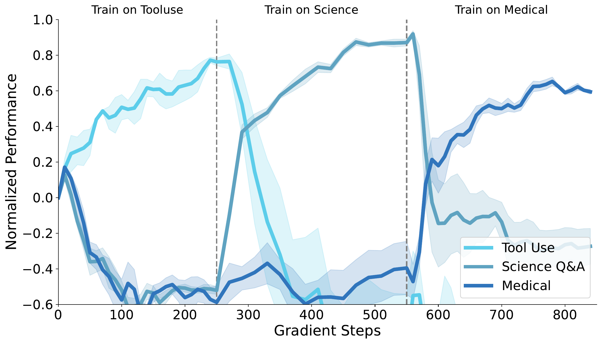
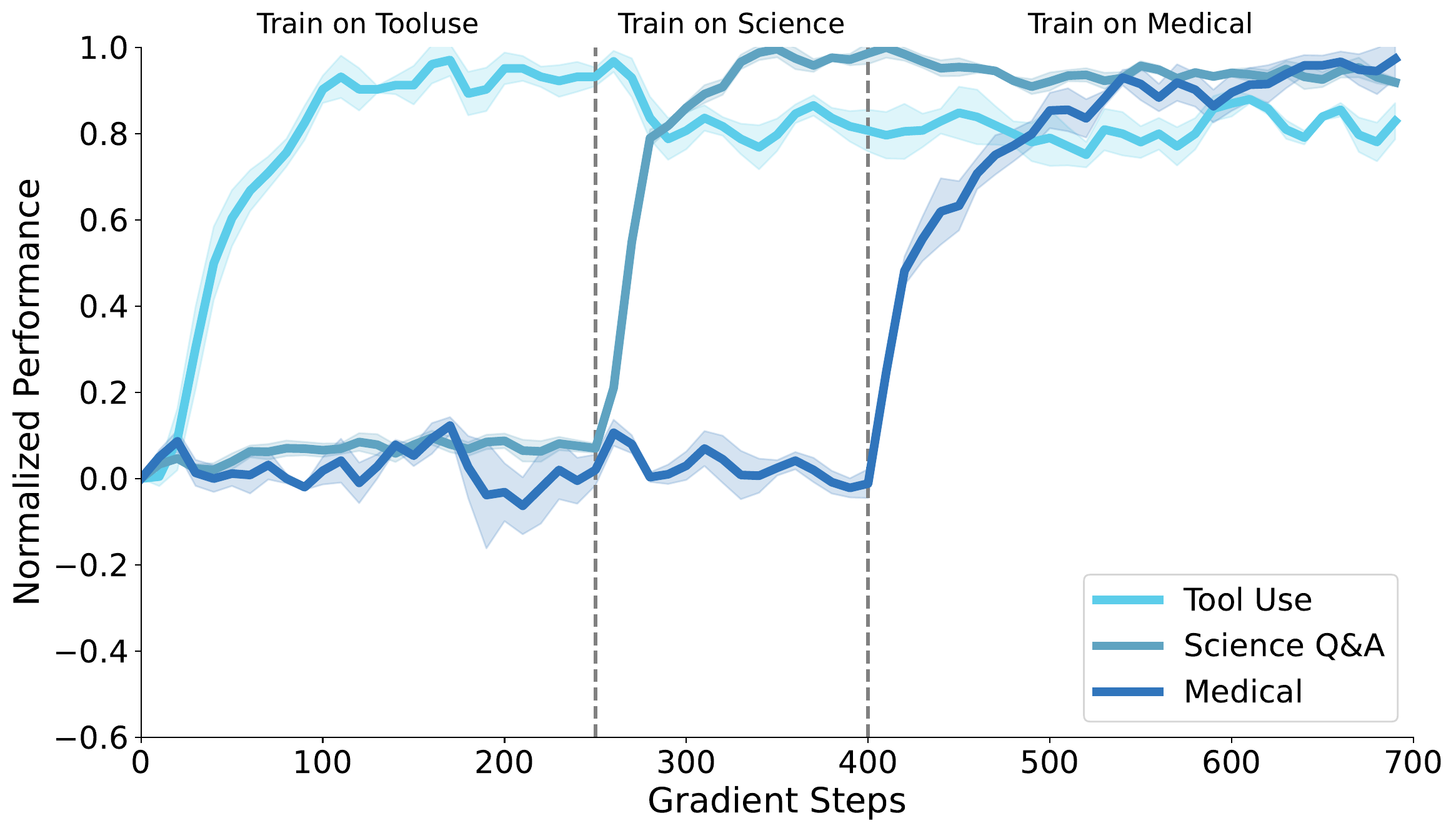
Train one model on Tool Use → Science Q&A → Medical. Normalize each task: 0 = base, 1 = best accuracy achieved by either method.

Figure 3a: sequential learning with SDFT
Figure 3a in the paper, SDFT. At each stage, new-task performance rises while earlier-task curves largely remain high.
Figure 3b: sequential learning with SFT
Figure 3b in the paper, SFT. After switching tasks, the previous task quickly falls below base (negative normalized score).

Only curves are given, without stage-end tables; shading shows variation across seeds. Normalization sets 1 to the best score across both methods, so heights are comparable only within each task.

Scale and pass@k: stronger ICL matters, beyond sharper outputs

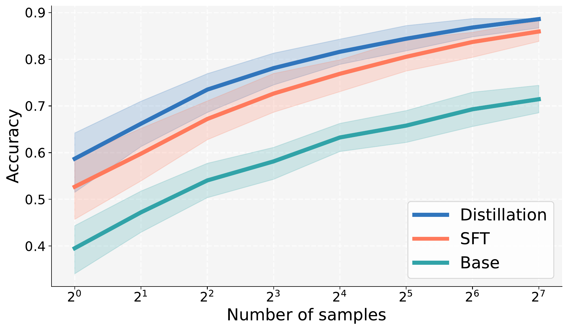
Scaling on Science Q&A; pass@k on Tool Use (temperature 1.0, top-p 0.95).

Model scale (Figure 5, left)

SDFT minus SFT on Science Q&A (points)

Qwen2.5-3B
−3.3
Qwen2.5-7B
+4.0
Qwen2.5-14B
+6.9

Axis: −14 to +14; vertical line = 0. The text reports only differences.

  • At 3B, weak teacher ICL makes SDFT worse than SFT.
  • The gap grows with scale; the authors expect more benefit from larger models.
  • Only three sizes, one task, and one model family are tested.

pass@k (Figure 5, right)

Figure 5 right: Tool Use pass@k
Figure 5, right, in the paper. For $k$ from 1 to 128, SDFT (Distillation) stays above SFT and base; the gap persists at larger $k$. A common concern is that RL improves pass@1 only by reducing entropy (Yue et al. 2025); these results do not support that explanation.

Knowledge acquisition nearly matches oracle retrieval

The base lacks these 2025 facts; SDFT absorbs them in a way that transfers to indirect questions.

Results (Table 1)

MethodStrictLenientOOD
Base000
Continual pretraining (CPT) on articles9377
SFT on question-answer pairs809580
SDFT8910098
Oracle RAG (upper-bound reference)91100100
  • CPT has little effect, consistent with Mecklenburg et al. 2024.
  • SFT reaches 80 strict accuracy but only 80 OOD: it reproduces answers without fully integrating the facts.
  • SDFT strict 89,OOD 98。

What must the teacher see? (Appendix A.2)

Strict accuracy (%) with on-policy training fixed and teacher context varied

Answers only
37
Articles only
75
Articles + answers
89
  • Earlier knowledge-injection self-distillation (Cartridges; Kujanpää et al. 2025) uses raw corpus context and offline training.
  • Adding worked answers to article context gains 14 points.

Answer-only data can adapt a reasoning model

SFT on short answers suppresses long CoT. SDFT's teacher is the same reasoning model, preserving its reasoning style in the target distribution.

Olmo-3-7B-Think, Medical (no CoT in the data)

Accuracy (%)

Base
31.2
+ SFT
23.5
+ SDFT
43.7

Axis: 0–100.

Mean response length (tokens)

Base
4612
+ SFT
3273
+ SDFT
4180

Axis: 0–5000 tokens.

Results

  • SFT reduces accuracy (31.2 → 23.5) and shortens responses by 29%, collapsing reasoning depth.
  • SDFT gains 12.5 accuracy points and retains 91% of the original response length.
  • Response length is used as a proxy for retained reasoning depth.

Implications

  • Real datasets often contain only final answers; closed models may not expose reasoning traces.
  • SDFT can adapt reasoning models to these data without reasoning demonstrations.

The reverse direction is difficult

In §5 the authors say converting a non-reasoning model to explicit CoT is difficult. SDFT can preserve a generation style, but cannot create a new one.

Gains come from on-policy training, beyond a better teacher

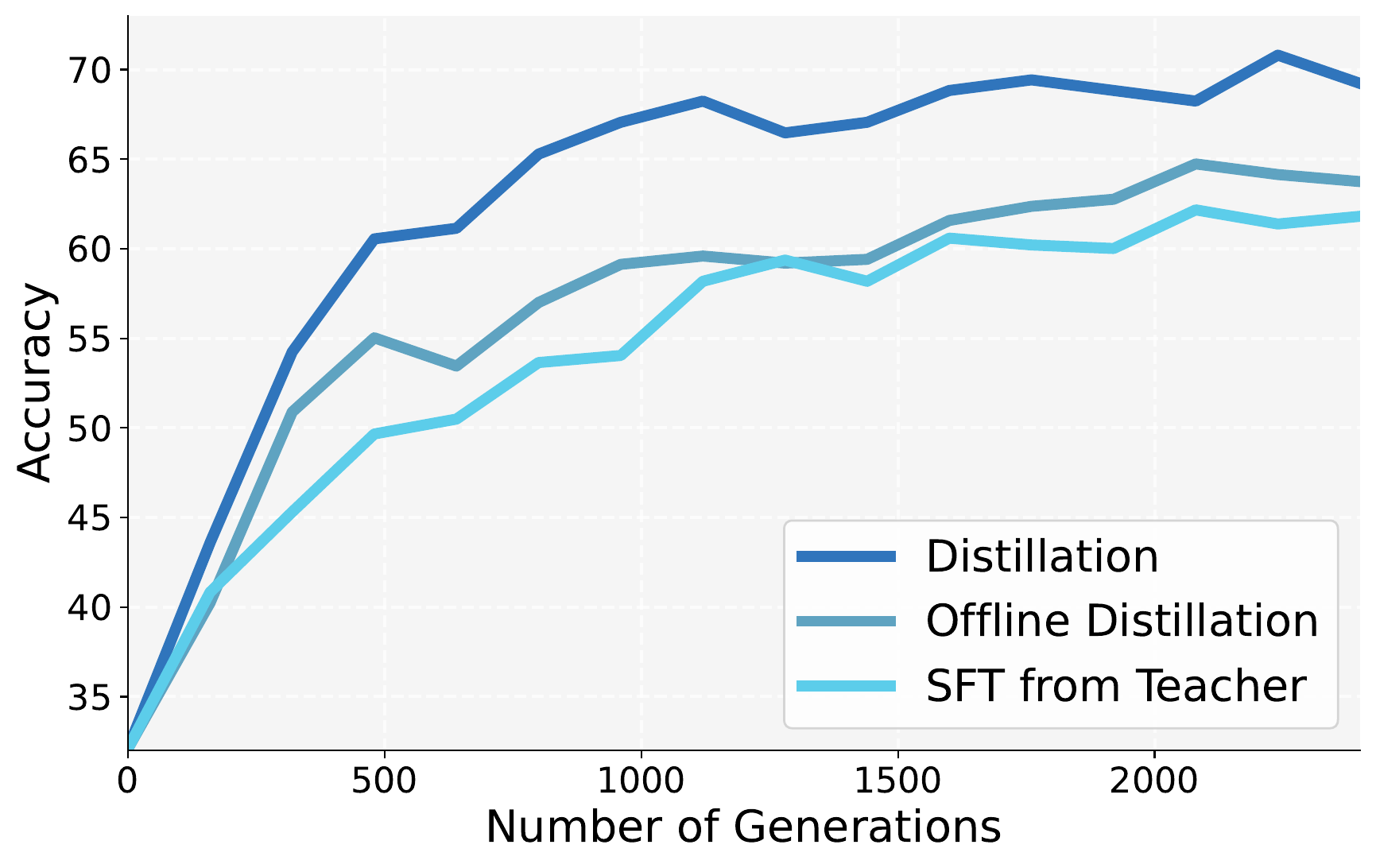
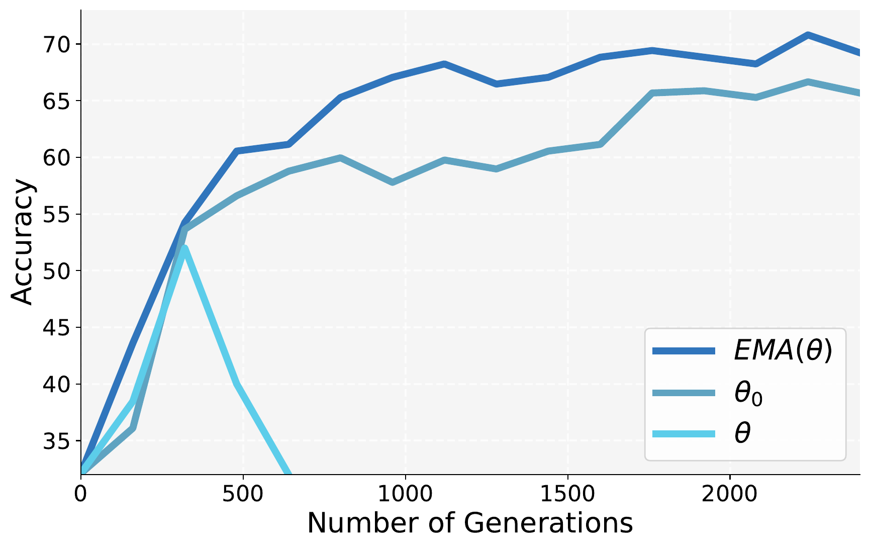
Figure 6 compares three uses of the same conditioned teacher; Figure 8 compares teacher weights. Both use Tool Use.

Offline vs on-policy (Figure 6)

Figure 6: on-policy versus offline distillation
Figure 6 in the paper. Distillation = SDFT; Offline Distillation = KL on fixed teacher outputs; SFT from Teacher = SFT on teacher samples. Both offline variants remain below SDFT throughout training.

Teacher weights (Figure 8)

Figure 8: teacher-weight ablation
Figure 8 in the paper. $\mathrm{EMA}(\theta)$ performs best; frozen base $\theta_0$ is stable but weaker; current student $\theta$ initially improves, then collapses midway.

Ablation summary

FactorFinding
Training distributionon-policy > two offline variants > SFT
Teacher weightsEMA > frozen base; current student diverges
Teacher contextarticles + answers 89 > articles 75 > answers 37
KL estimatoranalytic per-token best; no Rao-Blackwellized gain
Rollouts per query1 is enough
KL directionforward KL best (used for all results)
Model scale3B −3.3;7B +4.0;14B +6.9
EpochsSDFT 2 (skills) / 4 (knowledge); SFT no gain beyond 1

Figures 6 and 8 contain curves only (accuracy axis 35–70), without final numeric values.

Discussion and limitations (authors' statements)

SDFT complements on-policy RL when demonstrations are available but rewards are not.

Relationship to RL

  • Different supervision: demonstrations without rewards, versus rewards optimized through exploration.
  • Can combine: initialize RL with SDFT (supported by pass@k gains), or mix both signals.
  • Cheaper per step than GRPO: one rollout per query, with token- or even logit-level credit assignment.

Costs and failure modes

  • Compute: About 2.5 times SFT FLOPs and 4 times wall-clock time. Total time may be lower than SFT plus a recovery stage (e.g., Re-invoke).
  • Artifacts: Students imitate phrases such as "Following the example…"; masking early tokens is a heuristic fix.
  • Strong ICL required: fails at 3B.
  • Small behavioral changes only: cannot teach explicit CoT to a non-reasoning model.
  • Residual forgetting (e.g., IFEval 74.3 → 66.8 after Science Q&A).

Future work

  • Combine with on-policy RL: SDFT before RL, or jointly mix demonstration and reward signals.
  • Further reduce residual forgetting.
  • Learn from non-expert or noisy demonstrations.
  • Learn from unstructured data (e.g., user conversations) for real-world continual learning.

Summary: a demonstration-informed self supplies on-policy signals

These final two slides are our assessment, rather than the paper's statements.

Contribution

SDFT enables on-policy learning from demonstrations without rewards: on its own rollouts, the student distills from the same model (EMA weights) conditioned on demonstrations. On Qwen2.5-7B skill and knowledge tasks, it outperforms SFT on new tasks while largely retaining prior capabilities.

Findings to remember

  • Learn more, forget less: Tool Use 70.6 vs SFT 63.2; prior-task average 65.4 vs 56.0 (base 65.5).
  • Knowledge integration: OOD accuracy on injected facts 98 vs SFT 80, near oracle RAG's 100.
  • Answer-only reasoning adaptation: Olmo-3-7B-Think Medical 43.7 vs SFT 23.5; response length retains 91%.
  • On-policy is key: Offline distillation from the same teacher stays below SDFT (Figure 6).
  • ICL matters: SDFT trails SFT by 3.3 at 3B and leads by 6.9 at 14B.

Convincing evidence

  • Consistent reduction in forgetting: 3 tasks × 6 prior benchmarks; SDFT's prior-task average loses at most 1.0 vs base. TruthfulQA drops 7.7–11.1 for SFT/DFT, at most 1.4 for SDFT (Table 5).
  • Mechanism isolated: Figure 6 fixes the teacher and changes the training distribution, attributing gains to on-policy learning beyond teacher quality.
  • Ablated design choices: Teacher context (Figure 7), teacher weights (Figure 8), and KL estimator (Appendix A.1) have separate controls.
  • Beyond sharper outputs: pass@k consistently leads for $k\le 128$ (Figure 5, right).
  • Three sequential tasks show cumulative learning consistent with single-task results (Figure 3).

Critique: theory differs from training; broader transfer is unproven

Each point cites a specific section of the paper.

Thin evidence

  • Theory does not cover the actual loss: §3.1's IRL equivalence uses reverse KL, but all results use per-token forward KL (README, 2026-04-07); the analytic estimator is sequence-level biased (Appendix A.1).
  • One minimal-deviation measurement: 0.68 vs 1.26 nats, one task, against $\pi_0$ rather than each step's $\pi_k$ (§3.2).
  • Narrow scope: Mostly Qwen2.5-7B; scaling only on Science Q&A; only one reasoning model, Olmo-3-7B-Think.
  • Unmatched compute: SDFT uses about 2.5 times the FLOPs and 2–4 epochs; no compute-matched SFT or RL control.
  • Uncertainty not shown: Appendix B.2 says 95% CI over 3 seeds, but Tables 1, 2, 5 omit intervals.
  • Grading and retention metrics: Medical and knowledge tasks use GPT-5-mini grading; the prior-capability suite lacks math or long-reasoning benchmarks.

Open questions

  • Would reverse KL (matching the theory) give the same results? No direct forward/reverse comparison is reported.
  • At equal FLOPs, how does SDFT compare with more SFT epochs or RL when rewards exist?
  • Can the teacher prompt change a thinking model's reasoning style and distill that change into the student?
  • Does retention hold above 30B, across model families, and over longer task sequences?
  • With noisy or weak-model demonstrations, does the teacher still meet the optimality condition?

Our view: retention rests on a surrogate, and the anchor drifts

Left: the argument's core limitations. Right: directions worth testing.

Core limitations

  • A surrogate: "less forgetting" rests on an empirical correlation: forgetting grows with the KL between the fine-tuned and base models on new-task inputs (RL's Razor and others). SDFT minimizes student-to-teacher KL and lowers that quantity only indirectly, because the teacher stays close to the base. Both links are surrogates; this is the key limitation.
  • Measured in the wrong place: small KL on new-task inputs does not guarantee small KL on old-task inputs, which is what we care about. Parameters are shared, so a small change on new inputs can move outputs elsewhere.
  • The anchor moves: each step is a minimal change relative to the current policy $\pi_k$ (approximated by the EMA teacher), not the base $\pi_0$. A chain of small steps has no cumulative bound on $D_{\mathrm{KL}}(\pi_K\,\|\,\pi_0)$.

Directions to explore

  • An off-task anchor inside the loop. Mix retention prompts $x\sim\mathcal{D}_{\text{ret}}$ into training batches. New-task prompts use the EMA teacher as usual ($\mathcal{L}_{\text{SDFT}}$); retention prompts have no demonstration, where the EMA teacher is only a lagging copy of the student, so they anchor to the base $\pi_0$:
    $$\mathcal{L}=\mathcal{L}_{\text{SDFT}}+\lambda\,\mathbb{E}_{x\sim\mathcal{D}_{\text{ret}},\,y\sim\pi_\theta}\sum_t w_t\,D_{\mathrm{KL}}\big(\pi_\theta(\cdot\mid y_{\lt t},x)\,\|\,\pi_0(\cdot\mid y_{\lt t},x)\big)$$
    This constrains KL on old inputs directly and gives an anchor that does not drift with $k$. Baselines to beat: plain replay and LwF-style distillation.
  • Bonus: selective preservation. Not every base token on retention prompts is worth keeping; a per-position weight $w_t$ sets how strongly to preserve it. Heuristic: weight positions where the base is confident, e.g. $w_t=\exp\!\big(-H(\pi_0(\cdot\mid y_{\lt t},x))\big)$.
  • Closed-loop $\lambda$. Evaluate old tasks at a fixed interval and adjust $\lambda$ or the retention-prompt ratio. This batch-level control complements the token-level $w_t$.
  • Longer task sequences. Evaluate on sequences longer than the paper's three tasks and record when forgetting appears and which abilities it hits.